Introduction
This lab will introduce the concepts behind Satellite based Earth Observation or Remote Sensing, and the processing of Earth Observation data using cloud based computing platforms in particular Google Earth Engine.
The lab is aimed at the complete beginner both in terms of Earth Observation and cloud platforms and only requires access to an internet connected computer with a modern web browser such as Google Chrome.
At the completion of this lab you should understand the characteristics of the sensors used by Earth Observation satellites, how to visualise the information these sensors produce for simple processing and how to combine images taken over a period of time to remove cloud cover.
The Google Earth Engine Code Editor
You need to sign in to use Google Earth Engine which provides access to the imagery and cloud processing capabilities of the platform and also allows you to store the results of your analysis and share what you do with other users should you choose to – think of it like the Earth Observation version of Google Docs !
Visit code.earthengine.google.com using an incognito window on your browser and sign up using your existing Gmail or Google Account, if you don’t have a Google account yet ??? You can sign up for one by clicking on the Create Account ink.

The user interface ot Earth Engine has four main components along the top there are three panels which provide access to saved resources [A], an interactive text editor into which you will right code – Yes really [B] and finally a panel to display results of your processing [C].
The main part of the screen [D] is a map which looks like Google Maps, because it is ! This however is where the Earth Observation data we want to display will appear.
Pan and Zoom the map as you would using Google Maps to zoom into the South West of England with Exeter visible in the top right of the map like the diagram below..

For the rest of the lab we are going to concentrate on this part of England, so we need to be able to identify this particular part of the planet..
Using your mouse click on the Inspector tab in the upper right hand panel [B] and then click the mouse somewhere close to the centre of the map [D].
You should see something similar to this displayed

This is the location at the centre of the map screen and the level of zoom currently, for the moment just make a note of the centre point Longitude and Latitude – You only need to include the first three decimal points !
Just enough Javascript
Javascript is the scripting or programming language used by people who build websites so if should not be a great surprise to that it is used to control the Google Earth Engine, however don’t worry to complete the lab you only need to understand the very basics of Javascript.
Hello World
It is tradition that the introduction to any programming language is getting the worlds “hello world” printed on screen, so type the following text exactly as it is written below into the code editor panel [B] the upper middle panel.
// Hello world script
print('Hello World!');
As you typed you may and noticed that the editor tried to help my automatically closing brackets and changing the colour of the worlds as you type, this is called syntax checking and it’s the editor trying to stop you making mistakes – of course you will still be able to make mistakes otherwise where would the fun be…
The two forward slashes // mark the first line as a comment so the text after them is ignored by Earth Engine.
print(); is a function we are asking Earth Engine to print whatever we out inside the brackets in this case ‘Hello World” – It is very important to finish with a semicolon as this marks the end of the line of javascript and we can expect the script to be processed..
So to see if this works click on the run button and you should see the Console Tab in the upper right panel turn orange signifying there is something to look at, click on it and you should seen the following ..

Disappointed,, what did you expect fireworks !!
Variables and Objects
Lets try something a little more complex…
Click on the down arrow just to the right on the Reset Button and select “Clear Script”
Now type the following again exactly into the now clear code editor window..
var variable = 1;
var str = 'Hello, World!';
var centre = [-4.022, 50.591, 10];
var place = {
  name: "Exeter",
  population: 129800,
  county: "Devon",
  area: 47.04
};

print(variable);
print(str);
print(centre[2]);
print(place.name, place.county);
Once again click on the run button and look at your results in the console – All as expected ?
Let’s look at what you have done…
Var defines a variable or place holder, so in the first line you created a variable called variable and assigned it a value 1. Unlike some other programming languages you don’t need to specify that the variable in this case contains a number.
The second variable called str you assigned the contents ‘Hello, World” again you did not need to specify this is a string of text.
The third variable centre is a group or array of values from which we can chose a individual element so centre[2] is the value 10 – If this does not make sense think about how computers count ?
Finally the fourth variable is a key concept in javascript, as it is an object or dictionary. An object is a variable with named values known as properties or methods. So in this example place has the properties name, population, county and area. Any value may be identified as a name:value pair e.g place:county for Exeter is Devon.
Finally Functions
Often in programming you may want to do the same task or calculation many times, in javascript which can create a block of code to do a particular task again and again. Such a block of code is known as a function and in the example below we create a function to calculate population density.
var place = {
  name: "Exeter",
  population: 129800,
  county: "Devon",
  area: 47.04
};

function PopDen(pop, area) {
  return pop / area;
}

var x = PopDen(place['population'], place['area']);

print(x);
In this example the variable x stores the value of the function called PopDen which calculates population density when variables containing population and area are passed to it.
There are many predefined functions used to carry out all sorts of complex tasks in Earth Engine, you can spot them because they are usually called ee.something for example the function to load some earth observation data is ee.Image
OK that’s enough lets see some pretty pictures…
The height of Dartmoor in two lines…
Remember the Space Shuttle ? In February 2000 the Space Shuttle Endeavor captured a dataset of digital elevation in other words height using a specially modified Radar system known as the Shuttle Radar Topography Mission or SRTM.
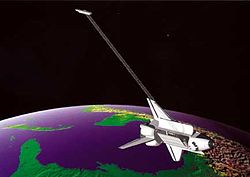
The United States Geological Survey processed the data over the next decade and in 2014 released a 30m grid cell version of the dataset, e.g the earth’s surface is divided up into cells or pixels of 30 x 30m (the size of a tennis court) and each cell is assigned a height.
Once again clear your code editor window and either type or cut and paste the following javascript exactly and press Run…
// Terrain Map.
var image = ee.Image("USGS/SRTMGL1_003")
Map.addLayer(image, {min:0, max:1000, palette: ["blue", "yellow", "red"]})
You should see the following..

You have defined a variable called image into which the function ee.image has loaded a version of the global SRTM dataset.
The Map.AddLayer function then displays the SRTM data on the map giving each pixel a colour depending on it height value using a colour ramp with blue representing low values passing through yellow to red representing high values.
You may have noticed that the image appeared in large squares, each square is the data coming from a different server. All the processing which takes place on Google Earth Engine is distributed meaning that different servers both process and store part of the data. This is what we mean when we talk about cloud processing, there are a cloud of servers !
Click on the Inspector tab once again on the upper right panel and try clicking at various points on the image you should see different elevation values in metres displayed.

Spend a minute or two sampling the elevation values and try to estimate the minimum and maximum values…
Now try modifying the code above to improve the visualisation, you want to try and achieve something that looks like this…

Eyes in the Sky
The earth has been observed from space on a regular basis since the early 1980’s, and unlike the imagery visible in Google Earth or Maps applications the observations have captured light reflected back from the surface of the earth across different discrete wavelengths many beyond what the eye can see. This is known as multispectral imagery and its use is key to the application of Earth Observation data from environmental monitoring, agriculture technology and resource exploration.
Materials reflect different amounts of light at particular wavelengths, for example in the visible part of the spectrum leaves reflect light mostly in the green part of the spectrum so they appear green, however beyond what the human eye can see plants reflect even more light in the near-infrared part of the spectrum. The difference in light reflected in the visible red and near infrared parts of the spectrum is known as the “red edge” and is very useful in identifying healthy crops.

The European Space Agency have launched a series of Satellites called Sentinels as part of the Copernicus programme and the data produced by these satellites is freely available on the Google Earth Engine platform.
In particular Sentinel-2 carries a multispectral sensor we are going to use in this Lab..
Clear the code editor window once again, and in the search bar at the very top of the screen type “sentinel-2”, and when is appears as in the diagram below click on “import”

This search bar allows you to both discover and access many petabytes of imagery, and is worth exploring later when you have the opportunity.
Import has created a variable containing in this case imagery produced by the multispectral instrument on the Sentinel-2 satellite, so to make things clearer rename the variable from the generic “imageCollection” to something more meaningful, for example Sen2

The multispectral instrument on Sentinel-2 can sense light reflected in 13 discrete wavelengths or bands, for this workshop however we are only interested in the first five…

In the code window enter the following code exactly and then press run..
var June = Sen2.filterDate('2018-06-01', '2018-06-15');

var rgb_vis = {
  min: 0,
  max: 3000.0,
  gamma: 1.5,
  bands: ['B4', 'B3', 'B2']
};

Map.addLayer(June, rgb_vis, 'RGB');
You should see something similar to this on the map screen..

So looking through the code what did you do to get this rather cloudy image;
The variable June defines a filter which creates a subset from all the possible images to select only those acquired during the first two weeks of June 2018.
The variable rgb_vis sets up the visualisation parameters that control how the data is displayed or rendered. We are letting Earth Engine know that the minimum value to expect is 0, the maximum 3000, to apply a correction of 1.5 and most importantly to use the data from bands 4,3 and 2 for this instrument that is the light reflected in the Red, Green and Blue parts of the visible spectrum.
Finally the function Map.addLayer is used to actually render the image using the two variables June and rgb_vis as passed parameters and displaying the 3 bands using Red, Green and Blue colours.
Because the light reflection in the Red, Green and Blue parts of the spectrum are displayed using Red, Green and Blue colours we get “True” colours displayed, in Earth Observation terms this is a True Colour Composite, Green things appear green, blue things appear blue !
More than meets the eye !
Click on the Inspector tab once again and inspect values around the image, there are a number of important points to note…

At each point three elements are return each of which can be expanded by clicking on the arrow.
Point gives you the location you clicked on and the size of each image element or pixel at the level of zoom you are using Google Earth Engineer is behind the scenes resampling the underlying images each time you zoom in and out to fetch only enough data to display on the screen. In this example each pixel in a square with sides 153m long.
Pixels provides the values representing the reflectance in each of the bands or channels the sensor has captured for this location.

Remember this is more than you are looking at, the display is using three bands but here you seen the data from all 13 possible bands.
Finally the object shows you actually how many discrete are available at this location. Remember a filter was used to set a window in time, the month of June in this case to select images from.

For this location in June 2018 there are actually three images available in the archive, what you see on the screen and the pixel values are from the latest image only.
This is really important the ability to look at a number of images of the same location over a period of time is a key strength of Earth Engine, looking at this type of data over time is known as multi-temporal analysis and in a little while we are going to use it to make the clouds disappear !
Spend a few moments looking at the values of different locations around the image, note that they may be some locations where there are more or fewer images available ?
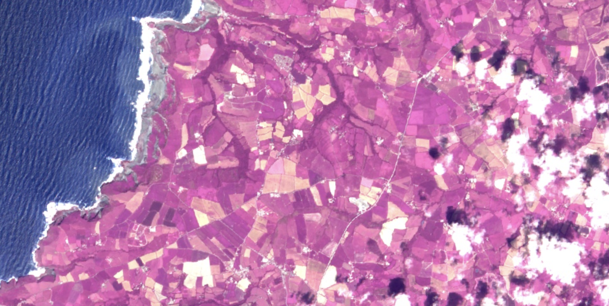
Seeing Red – False Colours !
One of the main ways Google Earth Engine is different of Google Earth is the ability to display and analyse all the data produced by Earth Observation Satellites, so far we have just replicated what we seen in Google Earth my creating a true colour composite image.
Instead of looking at the visible part of the spectrum, we can now start to use what is called the near infrared part of the spectrum, these are wavelengths of light where the leaves of healthy vegetation in particular reflect very strongly… For this particular satellite this is Band 5
As we are looking at wavelengths beyond those we can normally see it’s common to visualize this data differently… as we are most interested in near infrared we will display this band or channel using the red colour so areas of healthy vegetation will actually appear red on the screen rather than green.
See if you can modify the code you have used so far to add Band 5 instead of Band 2 and display it so that Band 5 is displayed as Red, Brand 4 Blue and Band 3 Green.
You should achieve something that is similar to this….

No more clouds
There are many quite sophisticated strategies which can be applied to use multi-temporal images to remove clouds however for this lab we are going to use a quick and dirty very simple method.
Looking at an image it is clear that the pixels with the highest values are those where they are clouds – clouds are very good at reflecting light across all wavelengths – so our simple approach is to look for each location in our area and across all the possible images available select the minimum number.
This is known as mapping a function e.g. we are carrying out the same function for every location in the image and is something that Earth Engine is very good at.
It is astonishing simple to do all we need to do is add the .min() function to Map.AddLayer…
Map.addLayer(June.min(), rgb_vis, 'RGB');
Try this and you should see some improvement…
There is one final parameter you may change to complete this lab and obtain the cloud free image from June 2018 below… but I will leave that to you to work out.
